Weighted Lloyd's Method for Voronoi Tesselation
This summer, I developed an algorithm to tesselate an image with Voronoi regions. I used a weighed Lloyd's method to distribute the Voronoi regions evenly throughout the image. You can now see the method on a dedicated static page.
The implementation is done entirely in JavaScript using the three.js library as well as dat.gui for exposing different parameters controlling the generated image.
After seeing a series of lectures given by Craig Kaplan on computational stippling methods, in particular on Weighed Voronoi Stippling, I gained an interest in applications for Voronoi diagrams. This gave me an idea to create an algorithm to crystallize an image using a collection of flat coloured Voronoi regions. Furthermore, I wanted the Voronoi regions to be evenly spaced, and I wanted more regions in detailed areas of the image. To get this effect I used a weighted Lloyd's method, where the weights are taken from the gradient of the image being tessellated.
Lloyd's algorithm
The basic Lloyd's method is simple. I will present the concept in the familiar 2D domain. First we define the Voronoi tesselation. Take a random set of \(n\) points, \( \mathcal{P} = \{\vec{x}_i\}_{i=1}^n \), where \( \vec{x}_i \in \mathbb{R}^2 \). Then the Voronoi tessellation generated by \( \mathcal{P} \) is the set of Voronoi regions \( \mathcal{V} = \{ V_i \} \) defined for each point \(i\) by $$ V_i = \left\{ \vec{x} \in \mathbb{R}^2 \mathrel{}:\mathrel{} \|\vec{x} - \vec{x}_i\| < \|\vec{x} - \vec{x}_j\|,\ \, \forall j\not=i \right\}. $$ The points in \( \mathcal{P} \) are called Voronoi sites. Furthermore, each Voronoi region has a centroid $$ C_i = \frac{1}{A_i} \iint_{V_i} \vec{x}_i\, d\vec{x} $$ where \( A_i = \iint_{V_i} d\vec{x} \) is the area of the Voronoi region.
Lloyd's algorithm consists of recomputing the Voronoi tessellation using the newly computed centroids as Voronoi sites. Repeating this process will spread the points evenly throughout the domain.
Since we are working in a pixelated domain, it is trivial to discretize the above integrals to compute region areas and centroids. Suppose \( p_k \) is the centre of pixel \( k \), and let \( N_i = \left|\{p_k \in V_i\}\right| \) approximate the number of the pixels covered by Voronoi region \( i \). Then the centroid of region \( i \) can be computed using the midpoint rule as \( c_i = \frac{1}{a_i}\sum_{p_k \in V_i} p_k \Delta x^2 \), where \( \Delta x^2 \) is the area of a pixel and \( a_i = N_i\Delta x^2 \) is the total area estimate. This simplifies to $$ c_i = \frac{1}{N_i}\sum_{p_k \in V_i} p_k. $$
Implementation
It remains to describe how we can determine if a pixel is in a Voronoi region computationally.
A standard method to visualize a Voronoi diagram is by rendering partially overlapping 3D cones aligned in a plane and all facing in one direction:
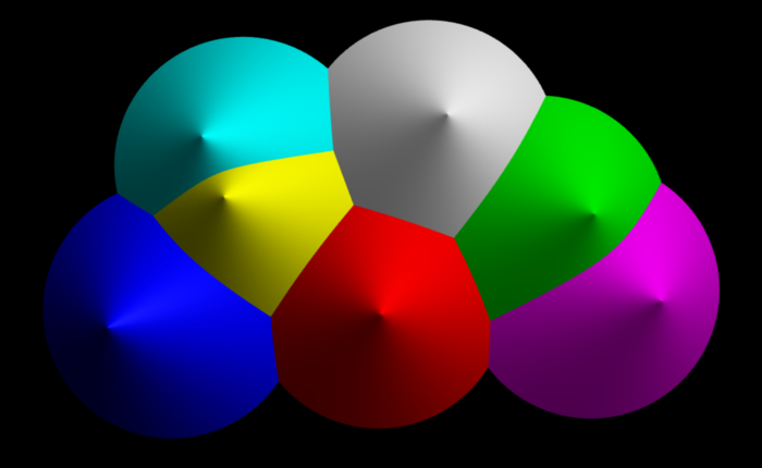
It should be clear from the image above that removing lighting effects and using an orthogonal projection (as opposed to a perspective projection) will effectively render a Voronoi diagram.
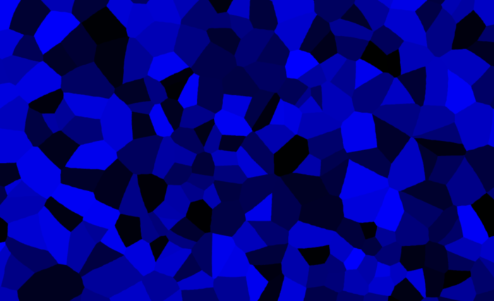
Finally, in order to compute the areas and centroids, we need to distinguish between different regions. This can be done by assigning a unique colour to each cone, which lets us to represent over 16 million regions if we use the standard web colours. Meaning that we can use a 24 bit number to be our identifier and interpret it as an RGB triplet when rendering the regions to a render target. We can then read the pixels from this target and determine which region they belong to. More specifically, given values \(r,g,b \in \{0..255\}\) read back from the render target, we can compute the identifier as $$ i = b + 256g + 256^2r. $$ The render target used for computation should look similar to this:
If you want to actually tesselate an image into Voronoi regions, then you can simply compute the average colour on each region as you iterate through the pixels of render target and the target image simultaneously. The average region colour is given by $$ r_i = \frac{1}{N_i}\sum_{p_k \in V_i} r_k $$ where \( r_k \) is the colour of \(k\)th pixel. This is done separately for all three colours (red, green and blue).
As an example we will use an image of Tux, the Linux mascot:

Using just Lloyd's method we can already get a nice crystallization effect:

Weighted Lloyd's Method
An interesting extension of Lloyd's method is moving the pixels into regions with a larger prescribed "density". In a sense we want to add a "bias" or "weight" to some areas of an image where we want more points to cluster. This is exactly the approach taken in Weighed Voronoi Stippling, except we will use a different weight. The motivation is that in areas of an image with more detail can benefit from a higher resolution or clustering of Voronoi regions. This can help direct the viewer's attention to more interesting areas of an image.
We start by assuming that we have a weight function \( w_k \in \mathbb{R}^+ \) that assigns each pixel \( k \), a positive real number. Then for each Voronoi region \( i \), we can compute a weighted centroid: $$ \tilde{c}_i = \frac{1}{W_i} \sum_{p_k\in V_i} w_kp_k $$ where \( W_i = \sum_{p_k\in V_i} w_k \) is the sum of all the weights. We can now use the weighted centroids \( \tilde{c}_i \) as the new Voronoi sites in the subsequent step in the algorithm to achieve the desired clustering.
Gradient Weight Function
The choice of the weight function determines the quality of region clustering. One possible way to cluster Voronoi regions near a highly detailed area is to weigh the centroids with the gradient of the image. In fact we only want the magnitude of the gradient. We can compute gradient in \( x \) and \( y \) directions at pixel boundaries by taking the difference of two pixel values. That is if \( I \) is our image function, then $$ \nabla I = \left(\frac{\partial I}{\partial x}, \frac{\partial I}{\partial y}\right)^T $$ is the gradient, where \( \frac{\partial I}{\partial x}\) can be descretized as \(\frac{I_{i,j} - I_{i+1,j}}{\Delta x} \) between pixels \((i,j)\) and \((i+1,j)\). Similarily we can compute the partial derivative in the \( y \) direction. We will then interpolate the gradient values to the pixel centers. A reader familiar with numerical differentiation will recognize this as the central difference approximation to each partial derivative. Finally, by taking the 1-norm of the result we get an approximation to the magnitude of the continous gradient:
$$ |\nabla I|_1 \approx \left|\frac{I_{i+1,j} - I_{i-1,j}}{2\Delta x} \right| + \left|\frac{I_{i,j+1} - I_{i,j-1}}{2\Delta x} \right| $$
Results
If the image has a sparse and sharp gradient (as it occurs in coarse drawings for instance), then the Voronoi regions will align with the boundaries in the image. With the gradient weighted Lloyd's method used on Tux, we get the following image:
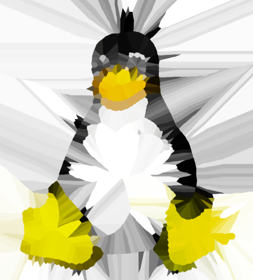
I chose this example specifically to emphasize the effect of the gradient weight. This is a drastically different image than the one using the vanilla Lloyd's method, but we need not stop here. We can add another step and blur the gradient of the original image to produce a smoother weight function. We can use any kind of blurring algorithm since we don't actually see the blurred gradient. I use the standard Gaussian blur to smooth the gradient (an efficient implementation can be found here). With a blur radius of 5 pixels we can achieve the following result:

Here we can see more clustering of Voronoi regions around the boundaries in the image, as compared to the crystallization using the unweighted Lloyd's method.
Applied to photographs, we can get nice stylized crystallizations, although the weights don't change the result much, since photographs are typically detailed everywhere:
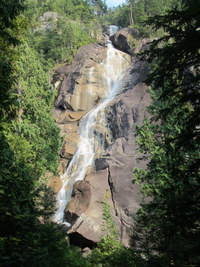
Original
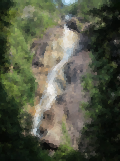
Crystallized
Final Thoughts
I'm rather surprised that this experiment turned out as well as it did. I found it particularly interesting how the Voronoi regions align to form the final configuration in a fluid-like manner. I would be interested to see how this animation will look when applied to a video sequence.